Examples

The central limit theorem

Let X be a Bernoulli random variable.

>>> import probly as pr
>>> X = pr.Ber()

We are interested in the sum of many independent copies of X. For this example, let’s take “many” to be 1000.

>>> num_copies = 1000
>>> Z = np.sum(pr.iid(X, num_copies))

The sum Z is itself a random variable, but its precise distribution, unlike that of X, is unknown.

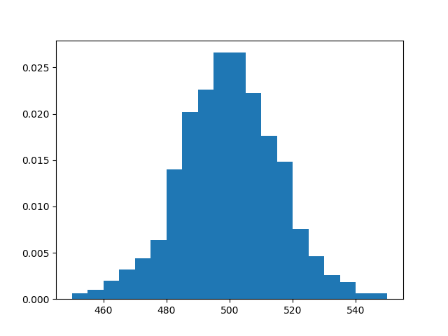
Nevertheless, the central limit theorem states, roughly, that Z is approximately normally distributed. We can check this empirically by plotting a histogram of the distribution of Z.

The more samples of Z we use to produce the histogram, the better an approximation it will be to the variable’s true distribution. But each time we sample Z, we must sample 1000 Bernoulli random variables and sum the results, so computing a histogram from very many samples can take a long time. Below we use 1000 samples, but you may want to reduce this number if running the code takes too long.

>>> pr.hist(Z, num_samples=1000)

The result resembles the famous bell-shaped curve of the normal distribution.

The semicircle law

A Wigner random matrix is a random symmetric matrix whose upper-diagonal entries are independent and identically distributed. We can construct a Wigner matrix using Wigner. For instance, let’s create a 1000-dimensional Wigner matrix with normally distributed entries.

>>> import probly as pr
>>> dim = 1000
>>> M = pr.Wigner(dim)

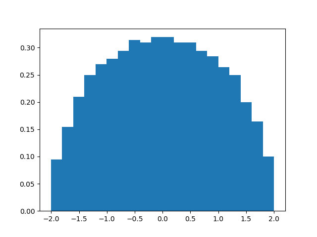
The semicircle law states that if we normalize this matrix by dividing by the square root of 1000, then the eigenvalues of the resulting (random) matrix should follow the semicircle distribution. Let’s check this empirically. First, we normalize M and then we construct its (random) eigenvalues by applying NumPy’s numpy.linalg.eigvals using lift().

>>> from numpy.linalg import eigvals
>>> M = M / np.sqrt(dim)
>>> eigvals = pr.lift(eigvals)
>>> E = eigvals(M)

The distribution of the eigenvalues can be visualized using the hist() function. Note that we need only take 1 sample.

>>> pr.hist(E, num_samples=1)  # doctest: +SKIP

Custom distributions

The following example shows how to create a custom distribution. We’ll start by constructing a simple non-random class.

>>> class Human:
>>>     def __init__(self, height, weight):
>>>         self.height = height
>>>         self.weight = weight

We’d like to create a kind of normal distribution over possible humans. We can do this as follows.

>>> import numpy as np
>>> from probly.distr.distributions import Distribution
>>> class NormalHuman(Distribution):
>>>     def __init__(self, female_stats, male_stats):
>>>         self.female_stats = female_stats
>>>         self.male_stats = male_stats
>>>         super().__init__()
>>>     def _sampler(self, seed):
>>>         np.random.seed(seed)
>>>         gender = np.random.choice(2, p=[0.5, 0.5])
>>>         if gender == 0:
>>>             height_mean, weight_mean, cov = self.female_stats
>>>         else:
>>>             height_mean, weight_mean, cov = self.male_stats
>>>         means = [height_mean, weight_mean]
>>>         np.random.seed(seed)
>>>         height, weight = np.random.multivariate_normal(means, cov)
>>>         return Human(gender, height, weight)

All the capabilities of random variables, including all those discussed above, will be available to our new random variable objects.

Note

Of course, certain operations may result in errors on sampling. For instance, sampling from the “sum” of two random humans will raise an error unless we overload addition for humans by defining __add__(self, other) in the Human class.

Let’s initialize an instance of this random variable.

>>> f_cov = np.array([[80, 5], [5, 99]])
>>> f_stats = [160, 65, f_cov]
>>> m_cov = np.array([[70, 4], [4, 11]])
>>> m_stats = [180, 75, m_cov]
>>> H = NormalHuman(f_stats, m_stats)

We can sample from and manipulate such a random variable as usual.

>>> @pr.lift
>>> def bmi(human):
>>>     return human.weight / (human.height / 100) ** 2
>>> BMI = bmi(H)
>>> BMI(seed)
23.57076738620301